Correlation plots with the "corrplot" Package

First, we load the packages "corrplot" and the data. You can easily access and download the dataset of this example following this link:

data_corr

.csv

Descargar CSV • 8KB

library(corrplot)
table_corr <- read.csv(file = "data_corr.csv", sep = ";")

We use the function "cor.mtest" to perform a significance test which produces p-values and confidence intervals for each pair of input features.

p.mat <- cor.mtest(table_corr)

The function "corrplot" is very easy to use and provides a lot of plotting options. "corrplot" has around 50 parameters, however the most common parameters are "method", "type", "order" or "diag" (see function details for further information).

corrplot(cor(table_corr,use = "pairwise.complete.obs", method='pearson'),method = 'number')

If we change the method...

corrplot(cor(table_corr,use = "pairwise.complete.obs", method='pearson'), method = 'circle')

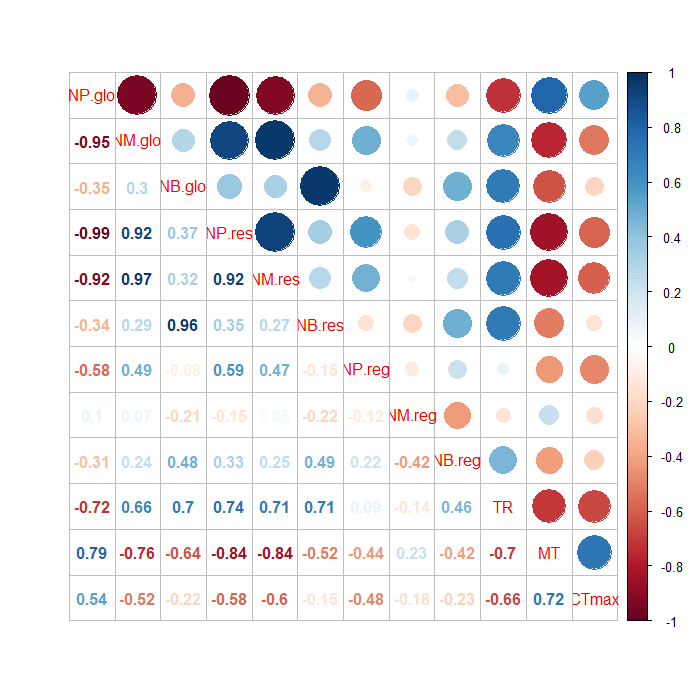
We can combine both methods using the function "corrplot.mixed".

corrplot.mixed(cor(table_corr,use = "pairwise.complete.obs", method='pearson'))

We can improve this plot modifying some addittional parameters.

corrplot(cor(table_corr,use = "pairwise.complete.obs", 
         method='pearson'),
         diag=F,tl.pos="lt",tl.col = 'black',method = 'number',
         col = colorRampPalette(c("#1874cd","grey60","#4A9022"))(200))
corrplot(cor(table_corr,use = "pairwise.complete.obs", 
         method='pearson'),
         type="lower", add=T, tl.pos="n", tl.col = 'black',cl.pos="n",
         col= colorRampPalette(c("#1874cd","grey60","#4A9022"))(200),
         p.mat=p.mat$p,sig.level = .05,
         insig = 'blank',  diag = FALSE)

As a result, we obtain a correlation plot showing Pearson's correlation coefficients above the diagonal. No circles are given for non-significant correlations (p > 0.05). We have changed the color palette and the color of the text.

Cano‐Barbacil, C., Radinger, J., Olden, J. D., & García‐Berthou, E. 2023. Estimates of niche position and breadth vary across spatial scales for native and alien inland fishes. Global Ecology and Biogeography, 32(3): 466-477. [link]