Create your own color palette in R

First of all, we load the packages "ggplot2", "scales" and "ggpubr".

library(ggplot2)
library(scales)
library(ggpubr)

We create a named vector ('mycolors ') with all the colors we want to include in our palette. To obtain a nice color combination you can use some webs like colorschemedesigner.com.

mycolors <- c(
  `green`= "#00B358",
  `light green`= "#62D99C",
  `dark green` = "#007439",
  `blue` = "#0969A2",
  `light blue` = "#64A8D1",
  `dark blue` = "#03436A",
  `yellowgreen` = "#74E600",
  `light yellowgreen` = "#B0F26D",
  `dark yellowgreen` = "#4B9500",
  `red` = "#FF3D00",
  `light red` = "#FF9473",
  `dark red` = "#A62800",
  `orange` = "#FF8C00",
  `ligth orange` = "#FFC073",
  `dark orange` = "#A65B00",
  `gold` = "#CFA127",
  `dark brown`= "#454416",
  `black` = "#000000",
  `light grey` = "#E6E6E6")
show_col(mycolors)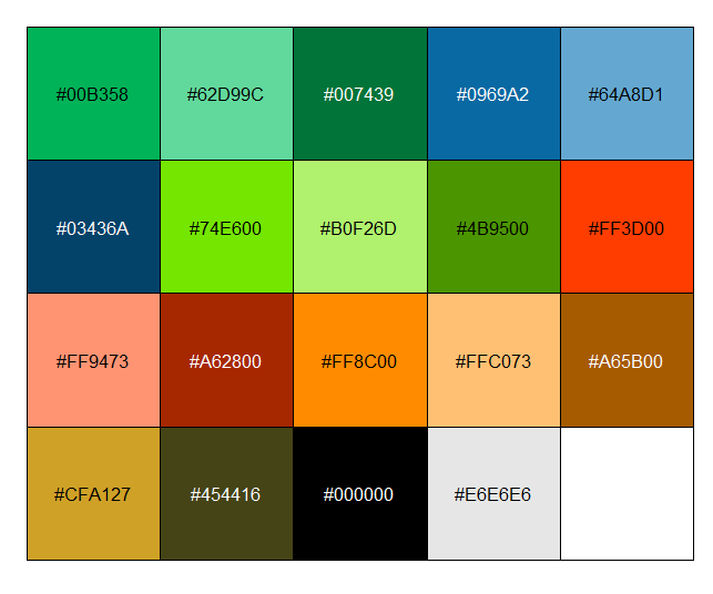

Next, we write a function called 'mycols' that extracts the hex codes from this vector by name.

mycols <- function(...) {
  cols <- c(...)
  if (is.null(cols))
  return (mycolors)
  mycolors[cols]
}

You can use this function to get hex colors in a very flexible way, and it’s also possible to use it manually in plots:

mycols("green")
#>    green 
#>    "#00B358"
mycols("green", "blue")
#>    green      blue 
#>    "#00B358" "#0969A2"
ggplot(iris, aes(Sepal.Width, Sepal.Length)) +
  geom_point(color = mycols("red"),
             size = 1.5, alpha =1)+
  theme_test()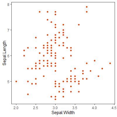

Now, we can start to combine our selected colors into different palettes (various combination of colors):

mypalettes <- list(
  `Tajo` = mycols("dark blue","green","light yellowgreen"),
  `Jarama` = mycols("dark brown", "green", "light yellowgreen"),
  `Manzanares` = mycols("blue","green","yellowgreen","orange","red"),
  `Culebro` = mycols("dark brown","orange", "light yellowgreen"),
  `Aphanius` = mycols("light blue", "gold", "dark brown", "black"),
  `Lepomis` = mycols("light blue","green","orange","black"),
  `Cyprinus` = mycols("black","dark brown","gold","light grey"))

Then, we write a function to access and interpolate them:

freshwater_pal <- function(palette = "Tajo", reverse = FALSE, ...) {
  pal <- mypalettes[[palette]]
  if (reverse) pal <- rev(pal)
  colorRampPalette(pal, ...)
}

This function allows to get a pallete by name from the list ("Tajo" by default). It also has a boolean condition determining whether to reverse the color order or not, and additional arguments to pass on to colorRampPallete():

freshwater_pal("Tajo")
#>    function (n) 
#>    {
#>        x <- ramp(seq.int(0, 1, length.out = n))
#>            if (ncol(x) == 4L) 
#>            rgb(x[,1L],x[,2L],x[, 3L],x[,4L], maxColorValue = 255)
#>        else rgb(x[, 1L], x[, 2L], x[, 3L], maxColorValue = 255)
#>    }
#>    <bytecode: 0x000000000c23d200>
#>    <environment: 0x0000000016033a70>

This returned function will interpolate the palette colors for a certain number of levels, making it possible to create new colors between our original ones. For example, we can interpolate the "Tajo" palette (which only includes three colors) to a length of 12:

colors <- freshwater_pal("Tajo")(12)
colors
#>    [1] "#03436A" "#025766" "#016B63" "#018060" "#00945C" "#00A859" #>        "#0FB859" "#2FC45D" "#50CF61" "#70DB65" "#90E669" "#B0F26D"
show_col(colors)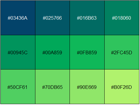

After that, we can create custom scales for ggplot2. We create one function for color and another for fill, and each contains a boolean argument for the relevant aesthetic being discrete or not:

scale_color_freshwater <- function(palette = "main", discrete = TRUE, reverse = FALSE, ...) {
  pal <- freshwater_pal(palette = palette, reverse = reverse)
  
  if (discrete) {
    discrete_scale("colour", paste0("freshwater_", palette), palette = pal, ...)
  } else {
    scale_color_gradientn(colours = pal(256), ...)
  }
}


scale_fill_freshwater <- function(palette = "main", discrete = TRUE, reverse = FALSE, ...) {
  pal <- freshwater_pal(palette = palette, reverse = reverse)
  
  if (discrete) {
    discrete_scale("fill", paste0("freshwater_", palette), palette = pal, ...)
  } else {
    scale_fill_gradientn(colours = pal(256), ...)
  }
}

Now, let's try our new palettes:

Tajo <- ggplot(iris, 
aes(Sepal.Width, Sepal.Length, color = Sepal.Length)) +
  geom_point(size = 2, alpha = 1) +
  scale_color_freshwater(discrete = FALSE, palette = "Tajo")+ 
  ggtitle("Tajo")+theme_test()+ theme(legend.position = "none")

Jarama <- ggplot(iris, 
aes(Sepal.Width, Sepal.Length, color = Sepal.Length)) +
  geom_point(size = 2, alpha = 1) +
  scale_color_freshwater(discrete = FALSE, palette = "Jarama")+ 
  ggtitle("Jarama")+theme_test()+ theme(legend.position = "none")

Manzanares <- ggplot(iris, 
aes(Sepal.Width, Sepal.Length, color = Sepal.Length)) +
  geom_point(size = 2, alpha = 1) +
  scale_color_freshwater(discrete = FALSE, palette = "Manzanares")+ 
  ggtitle("Manzanares")+theme_test()+ theme(legend.position = "none")

Culebro <- ggplot(iris, 
aes(Sepal.Width, Sepal.Length, color = Sepal.Length)) +
  geom_point(size = 2, alpha = 1) +
  scale_color_freshwater(discrete = FALSE, palette = "Culebro")+ 
  ggtitle("Culebro")+theme_test()+ theme(legend.position = "none")

Aphanius <- ggplot(iris, 
aes(Sepal.Width, Sepal.Length, color = Sepal.Length)) +
  geom_point(size = 2, alpha = 1) +
  scale_color_freshwater(discrete = FALSE, palette = "Aphanius")+ 
  ggtitle("Aphanius")+theme_test()+ theme(legend.position = "none")

Lepomis <- ggplot(iris, 
aes(Sepal.Width, Sepal.Length, color = Sepal.Length)) +
  geom_point(size = 2, alpha = 1) +
  scale_color_freshwater(discrete = FALSE, palette = "Lepomis")+ 
  ggtitle("Lepomis")+theme_test()+ theme(legend.position = "none")

Cyprinus <- ggplot(iris, 
aes(Sepal.Width, Sepal.Length, color = Sepal.Length)) +
  geom_point(size = 2, alpha = 2) +
  scale_color_freshwater(discrete = FALSE, palette = "Cyprinus")+ 
  ggtitle("Cyprinus")+theme_test()+ theme(legend.position = "none")

ggarrange(Tajo, Jarama, Manzanares,Culebro,
          Aphanius, Lepomis, Cyprinus, 
          labels = c("A", "B", "C","D", "E", "F", "G"),
          ncol = 4, nrow = 2)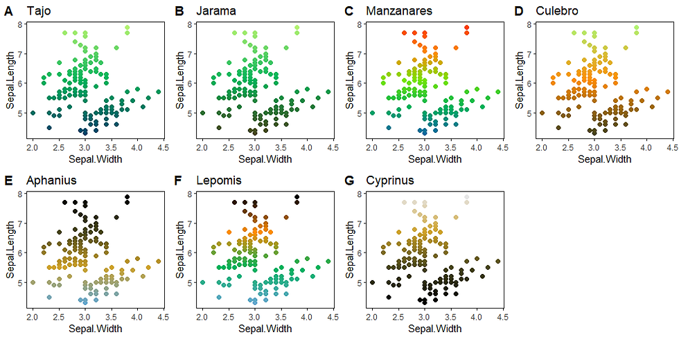

You can download and use all these palettes by installing the 'FreshWater' R package:

devtools::install_github("canobarbacil/FreshWater")
library(FreshWater)